Architecture AI Pathing Project: Upward Raycast for Better Opening Detection

January 11, 2021

Raycast for A* Nodes

Architecture AI Project


Original Downward Raycast and Downfalls

The raycasting system for detecting the environment to setup the base A* pathing nodes was originally using downward raycasts. These rays traveled until they hit the environment, and then set the position of the node as well as whether it is walkable or not. An extra sphere collision check around the point of contact was also conducted so as to check for obstacles right next to the node as well.

This works for rather open environments, but this had a major downside for our particular needs as it failed to detect openings with in walls and primarily doors. Doors are almost always found within a wall, so the raycast system would hit the wall above the door and read as unwalkable. This would leave most doors as unwalkable areas because of the walls above and around them.

Upward Raycast System Approach

Method

The idea of using an upward raycast was that it would help alleviate this issue of making openings within walls unwalkable when they should be walkable. By firing the rays upward, the first object hit in most cases can safely be assumed to be the floor because our system only works with a single level at this time. Upon hitting the first walkable target (in this case, the assumed floor), this point is set and another raycast is fired upward until it hits an unwalkable target. If no target is hit, this is determined as walkable (as there is clearly nothing unwalkable blocking the way), but if a target is hit, the distance between these two contact points is calculated. This distance is then compared with a constant height check and if the distance is greater, the node is still marked as walkable even though it eventually hit an unwalkable object.

This approach attempts to measure the available space between the floor and any unwalkable objects above it. If a wall is set directly onto the floor, as many are, the distance will be very small so it will not meet the conditions and will be set unwalkable appropriately. If there is a walkable door or just a large opening such as an arch, the distance between the floor and the wall above the door or the example arch way should be large enough that the system notes this area is still walkable.

Sphere Collision Check for Obstacles

Similarly to the original system, we still wanted a sphere collision check to help note obstacles very close to nodes so that the obstacles would not slip between the cracks of the rays cast, effectively becoming walkable. We included this similarly, but it is noted because the initial hit used is now below the floor, so the thickness of the floor must be accounted for. Currently a larger radius check is just needed so it can reach above and through the floor. In future edits, it could make sense to have a noted constant floor thickness and perform the sphere radius check above the initial raycast contact point according to this thickness.

Test Results

Details

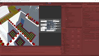
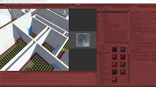
I compared the two raycast methods with a few areas in our current test project. In the following images, the nodes are visualized with Unity’s cube gizmos. The yellow nodes are “walkable” and the red nodes are “unwalkable”. Most of the large white objects are walls, and the highlighted light blue material objects are the doors being observed.

Test 1

A high density door area was chosen to observe the node results of both systems.

The downward check can work for doors when the ray does not directly hit a wall, as the sphere check properly checks them as walkable from the floor. However, the rays hitting the walls can be seen by the unwalkable nodes placed on top of them. A clear barrier is formed along the entirety of the walls, effectively making the doors unwalkable.

The upwards raycast test clearly shows every door has at least a single node width gap of walkable nodes in every case. The doors that were originally unwalkable with the downward raycast and now walkable as the height check was met.

Test 1: Downward Raycast


Test 1: Upward Raycast

Test 2

A larger room with a single noteable door was observed.

The downward check does pose a problem here as a full line of unwalkable nodes can be seen on the floor blocking access through the door and into the room. Because the problem is seen with nodes on the floor rather than nodes on top of the wall, this is actually a case where the sphere collision check is the problem and not the raycast particularly. Changing the collision radius for the check could potentially solve the issue here.

The upwards raycast is able to cleanly present a walkable path through this door into the room. While this does give us the result we desired, it should be noted again this difference can be attributed to the difference in the sphere collision check for obstacles. The same radius was used for both tests, but the upwards raycast sphere orginates from the bottom of the floor, so the extra distance it has to travel through the floor is what really opens up this path.

Test 2: Downward Raycast


Test 2: Upward Raycast

Summary

The upwards raycast seems extremely promising in providing the results we wanted for openings, doors especially. The tests clearly demonstrate that it helps with a major issue case the downward check had, so it is at worst a significant upgrade to the original approach. The upward raycast with distance check method also succeeded in other door locations, supporting its consistency. It will still have trouble from time to time with very narrow openings, but should work in a majority of cases.

via Blogger http://stevelilleyschool.blogspot.com/2021/01/architecture-ai-pathing-project-upward.html
Architecture AI Pathing Project: File Reader and Different Resolutions of Data and A* Pathing Grid

December 1, 2020

File Reader

Architecture AI Project


File Reader Data Array Creation

The file reader for this projects starts with the CSVReader class. This class is responsible for reading data in from .csv files generated by Revit to pass it on to the underlying A* pathing node grid for use by the agents when pathing. These .csv files have 2D coordinate values to locate the data, the actual data value, and a reference ID. The coordinate data and the data values themselves are separated and saved into many data objects within Unity (in a class named DataWithPosition). This prepares the data to be used to pass on to the A* pathing node grid.

While the .csv data is generally consistently spaced based on coordinates, it can have many gaps as it does not assign a value somewhere where there is a gap in the model. This results in data that is not perfectly rectangular. To make the process of tying this data array in with the pathing grid more consistent, I manually make a rectangular data array to hold all of the data and fill in the missing coordinates with additional data objects that have some default value (usually “0”). This helps fill the data into the A* pathing grid as the grid is created because it can simply go through the data list one at a time instead of doing any searching of any kind.

Applying the Read Data to the A* Pathing Grid

Data Assumptions:

  • In order by coordinates, starting with the x-coordinates
  • There is a general consistent distance between the data points

After reading in all the data and creating the foundational array of data, it can then be applied to the node grid. The first basic case of this reads through the data array as A* pathing grid is created and assigns values as the grid is made. This however only makes sense when the resolution of the data being read in and the A* pathing grid are similar. If there is a substantially higher density of data points, or a higher density of node grids, this is no longer the case and we need other ways to apply the data.

Data Resolution Cases

This leads to three cases (Cases with respect to data resolution):

  1. Data Resolution = A* Pathing Grid Resolution
  2. Data Resolution > A* Pathing Grid Resolution
  3. Data Resolution < A* Pathing Grid Resolution

(The 3 cases with respect to distance):

  1. Data Distance = A* Pathing Grid Node Diameter
  2. Data Distance < A* Pathing Grid Node Diameter
  3. Data Distance > A* Pathing Grid Node Diameter

The resolution here is the inverse of the distance between the data points (i.e. the distance between the data point coordinates, and the node diameters). This also means these cases can be checked based on the distance between data points as well, but the condition is reversed (except for the case where they are equal, where it stays the same).

Determining which case is present is important to determine how to apply the data to the A* pathing nodes. I determined the best way to deal with these cases in a simple manner was the following:

Dealing with the 3 Cases of Data Resolutions

Dealing with the 3 Cases:

  1. Similar Number of Data Points and A* Nodes: Apply data to the A* pathing nodes 1-to-1
  2. Substantially More Data Points than A* Nodes: Average the data value of all the data points covered by each A* node for each A* node
  3. Substantially Less Data Points than A* Nodes: Apply the same data value from each data point to all the A* nodes in the same area it covers

These other cases require additional information to accurately apply these various techniques. Adding an additional data assumption that when there is a difference in the distance between data points and the A* node diameter that this difference such that the distances are divisible by one another leads to a useful term that can consistently help with both of these cases.

If (distance between data is divisible by A* node diameter OR A* node diameter is divisible by distance between data)

To keep it somewhat consistent, I created a term called the “Distance Ratio (D)”, which is the node diameter divided by the distance between the data point coordinates. This term can be used as an important data dimension when dealing with array indices for the different data application cases. Since the key is using this as a dimensional property, it needs to be a whole number, which is not the case when the node diameter is less than the distance between data coordinates. In this case, the inverse of “D” can be used to find the dimensional term.


Distance Ratio (D) = Node Diameter / Distance Between Data

Dimensional Ratio (D*)

if (D >= 1) D* = D

if (D < 1) D* = 1 / D

Using Dimensional Ratio for Cases 2 and 3

Case 1 does not need the dimensional ratio whatsoever, but both other cases can use it.

Case 2

For case 2 there are more data points per area than A* nodes, so the A* nodes must average the value of all the data points they cover. These data points can be found using the dimensional ratio. Each A* node covers a number of data points, n, where (n = D* ^ 2). This information makes it much easier and more consistent to find the proper data to average while setting the values during the creation of the A* node grid.

Case 3

For case 3, there are less data points than there are A* nodes in each given area. Since this case just applies the same value from a given data point to several A* nodes, it is just about figuring out all the A* nodes each data point should pass its data to. This can also be done by expanding the initial data array out with a bunch of identical data points so that it can then follow the 1-to-1 passing on approach of case 1.

To do this, the dimensional ratio, D*, is used again. The initial data array created from the reading of the .csv file can be modified and expanded. A new 2D data array is created with each dimension (height and width) multiplied by D*. Then each data point passes on all of its information to a square of data points in the new array, where the number of new data points created, n, is such that (n = D* ^ 2).

File Reader Data Resolution Difference Summary

This allows us to deal with various types and sizes of data while using various resolutions of A* pathing node systems somewhat consistently. This can be beneficial when passing in many types of data that could have different data resolutions and you want to keep the A* node grid resolution consistent. This also just helps the system perform properly when many types of data are passed through it over the course of several tests.

Unfortunately the distance between the data points is not determined automatically at this time, so it must be input manually. I initially thought of just finding the difference between the first couple coordinates to determine the distance, but this would fail edge cases where some of the data right at the beginning is missing. The better solution could be to randomly select several pairs of coordinates throughout the data and find the difference, then use the mode of that data as the determined data distance. This would work in most cases, and could then just have a manual override for fringe cases.

Case 3 in particular is definitely not the most efficient approach, but it was a quicker and simpler implementation for now. Ideally it would not need to create another expanded data grid as a reference, and the A* node grid could use some method to know which ones should read from the same data point.

Next Step

This process could benefit from some of the possible updates mentioned in the “File Reader Data Resolution Difference Summary” section, but most of those should be unnecessary for now. The next steps will look to other parts of the system, which does include some more file reading that some of this process could benefit. We need to read in more Revit data to assign data to the model objects themselves.

via Blogger http://stevelilleyschool.blogspot.com/2020/12/architecture-ai-pathing-project-file.html

Architecture AI Prototype Historical Path Visualization and UI Updates

July 1, 2020

Architecture AI Project

Added Path Visualization and UI Updates

Introduction

To top off the prototype, we added a quick visualization tool to show any paths that agents have taken within the current game session. This was necessary to make it easier to compare the paths of various combinations of agents and environments even. Along with this, some elements of modifying the system that were only accessible within the Unity Inspector have been moved to the in game UI. This makes it much more manageable to alter the agents and their pathing for Unity users and non-users alike.

The following quick reference image shows an example of this new path visualization tool (the red line going through the diagonal of the area).

Reference for New Path Visualization Tool (the Red Line is the Path)

Vimeo – My Demo of the Past Path Visualization Tool (with New UI Elements)

Past Path Visualization Feature

Visualization

The path data was already being recorded in an in-depth manner for storing the data in a text format for export, so here we just focused on using that data during the game session to provide another useful data visualization tool. This data is kept as an array of Node objects, which in turn individually hold information on their world position. This provided a solid foundation to visualize the information again.

The array of Nodes could then provide me with an array of world positions which I could use with Unity’s line renderer to create a basic line connecting all of these points. Using the line renderer component also leaves the tool flexible through the Inspector to modify how the line is drawn to fit different needs or environments.

Dropdown UI

To make this easy to access for the user, I added a Unity dropdown UI element to the scene to hold information about all the past paths. It initializes by creating a newly cleared dropdown and adding a simple “None” option which helps keep everything in line, as well as providing the user an obvious spot to go back to when they don’t want to show any previous paths. Then as paths are generated, more options are added to this dropdown to keep it in line with all the paths created (this also keeps their indices in sync for easy reference between the dropdown and the recorded paths).

Added UI Elements for Operating System

As a prototype tool, a quick way to allow for tweaking values and controlling assets is to just use public variables or Unity tool assets (like Unity Ranges and enums within the scripts). This became even cumbersome for myself, so it could be a large issue and slow down for less savvy Unity users. This made me want to explore moving some of these parameters into the game UI for easier use.

Agent Affinity Sliders

I looked into creating Unity UI sliders and since there were pretty easy to implement I moved the range sliders from the Unity Inspector for setting the different agent affinities for the next spawned agent to the game UI. This was straightforward in that the slider values could almost directly be transferred to the spawnmanager (The slider actually goes between values of 0.0 – 1.0 and is multiplied by the max affinity value of the system to properly stay constrained within that range).

Agent Pathing Type Dropdown

After exploring the dropdowns for the path history visualization tool, I also decided to use them for determining the path type of the next spawned agent. This allows the user to quickly choose between different architectural types to use to calculate the agent’s pathing.

Since the architectural types are within a public enum, the dropdown could be populated by the ToString() versions of this entire enum (which can be cycled through in C#). Since they are populated this way in order based on the enum itself, the dropdown can inform the PathFindingHeapSimple (the class that needs to know the type in order to determine which pathing calculations to use) based on the enum index number. They should be kept in sync based on the way the dropdown is created.

Summary

The past path visualization tool is very useful for comparing paths a bit more quickly (since changing values for individual paths can take a small bit of time). It may help in the future of the project to visualize multiple paths at once to directly compare paths very easily. The system also displays information about the path it is showing so the user knows better why the path is the way it is.

Unity’s UI elements are pretty easy to work with, and adding methods to their OnValueChanged delegate is a very nice and consistent way of only calling changes/methods specifically when a UI element is modified. This was perfect for both the dropdowns and the sliders since they only need to invoke change within the system when their values are changed. This keeps them a bit cleaner and more efficient.

The UI elements are strongly tied to the borders of the screen using the standard Unity positioning constraint system, so it can look really messy at smaller resolutions. It operates well enough since there’s not too much going on, so just allocating a decent resolution to the window when using it at least shows everything which is the most important aspect for a prototype.

Architecture AI Completed Prototype with Data Visualization and Pathing Options

June 24, 2020

Architecture AI Project

Completed Project Prototype

Introduction

We were exploring different methods for importing architectural models into Unity and decided to try Revit to see what it had to offer. The models are easy to move between softwares, and it also creates .cs scripts that Unity can use to provide some interactive data visualization when using the Revit models.

Data Visualization Options

I moved everything dealing with the major logic of the A* grid node visualization into its own class named AStarGridVisualization. This allowed me to continue to hold on to all the different debug visualization methods I created over the course of the project and convert them into a list of options for the designer to use for visualization purposes.

As can be seen in the demo, there is a list of options in the drop down list in the Unity Inspector so the designer can tell the system which data to visualize from the nodes. The options currently available are: Walkable, Window, and Connectivity. Walkable shows which nodes are considered walkable or not. Window and Connectivity show a colored heat map to show those respective values within the nodes themselves.

Changing Values Used for Pathing

The project wanted to be able to use different types of values to see their effects on the agents’ pathing, so every node has several different types of architectural values (i.e. Window and Connectivity). Using the window information for pathing will give different agent paths than when using the connectivity values, because the agents have different affinities towards these types of values and the nodes have different values for these different types contained within the same node.

The PathFindingHeapSimple class handles the calculations for the costs of the paths for the agents, so I have also located the options to switch between pathing value checks here. This class is responsible for checking nodes and their values to see which lead to the lowest cost paths, so there is another drop down list available to the designer here that determines which architectural value type these checks look at when looking at the nodes. This allows the designer to choose which architectural value actually influences the agents’ paths.

A* Node Grid Construction Options

This point of the project was still working with various types of model imports from various softwares to find which worked the best and most consistent, so I added some extra options for generating the node grid in the first place to give some quick options that may better help line up the node coverage area with the model at hand. These major options located in the AGrid class itself are: GridOriginAtBottomLeft and UseHalfNodeOffset (the third is determining whether the system reads data from a file or not to add values to the node grid, but that’s a more file oriented option).

GridOriginAtBottomLeft

GridOriginAtBottomLeft determines where Unity’s origin is located relative to the node grid. When true, Unity’s origin is used as the bottom left most point of the entire node grid. When false, Unity’s origin is used as the central point of the generated node grid.

UseHalfNodeOffset

UseHalfNodeOffset is responsible for shifting the nodes ever so slightly to give a different centering option for the nodes. When true, half of the dimension of an individual node is added to the positioning vector of the node (in x and z) so that the node is centered within the coordinates made by the system. When false, the offset is not added, so the nodes are directly located exactly at the determined coordinates.

File Reading to Set Values Within Nodes

There are two major ways to apply architectural values to the nodes: using architectural objects (within Unity itself) or reading data from a file. The data files contain x and y coordinate information along with a value for a specific architectural value for many data points throughout a space. These files can be placed Unity’s Assets/Resources folder to be read into the system. The option referenced above in the AGrid to read data from a file or not is the IsReadingDataFromFile bool, and it just tells the system whether or not to check the file told to the system to assign values to the grid.

The FileReader object holds the CSVReader class which deals with the logic of actually reading this file information. The name of the file to be read needs to be inserted here (by copy/paste generally to make sure it is exact), and the dimensions of the data should be manually assigned at this time to make sure the system gets all of the data points and assigns them to the grid appropriately (these data dimensions are the “x dimensions” and “y/z dimensions” ranges of the coordinates within the data).

Demonstration of Prototype

This demonstration helps show the different data visualization options of the grid, the agent spawning system, how changing the architectural value path type changes the agents’ paths, and how a lot of these systems look in the Unity Inspector.

Vimeo – Architecture AI Project Prototype Demonstration

Summary

I really liked a lot of the options I was able to add to help increase the project’s overall usability and make it much easier to switch between various options at run time to test different setups. The end product is meant to help users that may not have a lot of Unity experience, so I tried to reduce the learning curve by making a lot of options easily accessible with visible bools and drop down lists, while also providing some simple buttons in the game space to help with some other basic actions (such as spawning new agents).

Many of the classes were constructed with scalability and efficiency in mind, so expanding the system should be very doable. However much of this scalability is still contained within the programming itself and the classes themselves would need to be modified to add more options to the system at this point (such as new architectural types). This is something I would like to make more accessible to the designer so that it’s intuitive and possible to modify without programming knowledge.

The file reading system works well enough for these basic cases, but it could definitely use some work to be more flexible and work with various node grid options. This is something I could use more work on in general, and having systems to read in files and output files to record data would be useful to understand better in general.

Architecture AI Varied Agent Affinities with Varied Pathing

May 28, 2020

Architecture AI Project

Varied Agent Affinities with Varied Pathing

Demonstration of Varied Agent Affinities with Varied Pathing

Vimeo Link – My Demo of Agents Pathing with Varied Affinities

Explaining Simple but Unclear Heatmap Coloring System

Just to help explain since I don’t have great UI in to explain everything currently, the first thing was that I was testing a really rough “heat map” visual for the architectural values for now. When you turn on the option to show the node gizmos now, instead of uniform black cubes showing all the nodes, the cubes are colored according to the architectural value of the node (for this test case, the window value) Unfortunately this color system isn’t great, especially without a legend, but you can at least see it’s working (I just need to pick a better color gradient). Red is unfortunately both values at/near 0 (min) as well as at/near 100 (max) (but the value range here is only from 0 – 80, so all red in this demo is 0).

Agent Affinity/Architectural Value Interaction for Pathing

The more exciting part is that the basis of the agent affinity and architectural value interactions seem to be working and affecting their pathing in a way that at least makes sense. Again just for demo purposes so far, as can be seen in the video (albeit a bit blurry), I added a quick slider on the inspector for the Spawn Manager to determine the “Window Affinity” for the next agent it spawns (for clarity I also added it as a text UI element that can be seen at the top of the Game View window). Just to rehash, this has a set range between 0 and 100, where 0 means they “hate” windows and avoid them and 100 means they “adore” windows and gravitate towards them.

Test #1: Spawn Position 1

As can be seen in the first quick part of the demo, I spawn 2 agents from the same position 1 but with different affinities. The first has an affinity of 0, and the second has an affinity of 100. Here you can already see the 0 affinity agent steers towards the left side of the large wide obstacle to avoid the blue (relatively high) window area, where as the 100 affinity agent goes around the right side of the same obstacle, preferring the high window valued areas in the blue marked zone.

Test #2: Spawn Position 2

Both the 0 affinity and 100 affinity agents take very similar path, differing by only a couple node deviations here and there. This makes sense as routing around the large high window value area would take a lot of effort, so even the window avoidant agent decides to take the relatively straight forward path over rerouting.

Test #3: Spawn Position 3

This test demonstrated similar results to that of Test #1. The 100 affinity agent moved up and over the large obstacle in the southern part of the area (preferring the high window value area in the middle again), where as the 0 affinity agent moved below the same obstacle and even routed a bit more south just to avoid some of the smaller window afflicted areas as well.

Summary

I did some testing of values in between 0 and 100 and with the low complexity of the area so far, most agents ended up taking one of the same paths as the 0 or 100 affinity agents from what I saw. This will require more testing to see if there already exists some variance, but if not, this suggests that some of the hardcoded behind the scenes values or calculations for additional cost may need tweaked (as is expected). Overall though, the results came out pretty well and seem to make sense. The agents don’t circle around objects in a very odd way, but they also do not go extremely out of there way to avoid areas even when they don’t like them.

Architecture AI Heatmap of Architectural Costs

May 27, 2020

Architecture AI Project

Visualizing Heatmap of Architectural Costs

Architectural Cost Heatmap

I was just using basic black cubes to visualize the grid of nodes in the AGrid A* system originally. Now I finally decided to update that system with a bit more information by adding a colored heatmap to map out the architectural values of the nodes. This will help me understand the pathing of my agents better as they start to use these values in more complex and interesting ways.

Basic Heatmap Color System

It turns out making a heatmap color scale that decently ranges between values of 0.0 and 1.0 is pretty easy. Using HSV color values, you can just vary the H (hue) value while keeping the other two values constant at 1.0 to cover a heatmap spectrum (where H of 0.0 is the lowest value in the range, 1.0 is the highest value in the range, and all other colors are bound within that range). By simply using the min and max architectural values possible in the system as the range bounds I could easily set this type of system up.

Applying Colors to Visualization

For now I decided to just apply this heatmap color methodology to the cubes mapping out the A* grid for now. While these gizmo cubes used to just be colored black for simplicity, now they are colored according to the heatmap color system using the architectural value found within the node.

Bug: Influence Objects Found to Radiate Improperly

The influence objects which apply architectural values to the nodes around them were initially designed to apply in an area around them, with the objects in the center. After applying the heatmap, it was clear that the influence objects were not applying to the nodes intended. It appears the influence actually uses the position of the influence object as the bottom left corner, and radiates upward and to the right (so just in the positive x and z direction away from the object). This is something I will have to look into to make sure it’s an issue with the influence objects, and not the coloring system.

Current Heatmap System (with Bugged Influence Ranges)

AGrid Inspector Breakdown for A* Pathfinding

May 5, 2020

A* Pathfinding

AGrid Inspector Breakdown

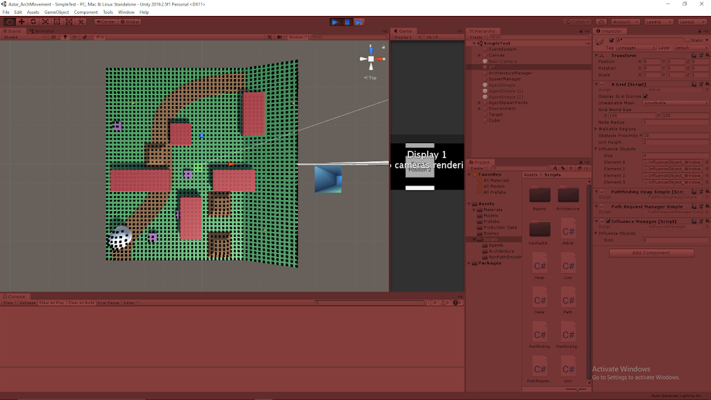
Display Grid Gizmos:
determines whether or not to run gizmo methods (methods used for debugging and visualization in the editor, like the node locations)
Unwalkable Mask:
this is the Unity layer that is deemed unwalkable to the system (the layer which are picked up by the nodes during raycasting)
Grid World Size:
a Vector2 which determines the real world size area to attempt to place nodes on (rectangular shaped with alterable width and height)
Node Radius:
half the real world size of each individual node, which correlates to half the distance between each node’s center (in both the x and z direction)
Walkable Regions:
this section can be opened and various terrain types can be added to this as well as their associated movement cost penalties to make certain terrains more or less navigable (also picked up in the raycast of the nodes)
Obstacle Proximity Penalty:
adds a bit of extra cost to nodes right around obstacles to make agents less likely to run right up against (or right inside) of obstacles
Unit Height:
currently used in conjunction with system placing the nodes at the proper elevation to place nodes slightly above the terrain so that using those location as waypoints for the agents does not make them go through/below the ground
Influence Objects:
variable sized array that can be filled with Influence objects so system knows which Influence objects to apply when filling out node values

Example Images of AGrid System and Inspector Designer Tools

Fig. 1: Visualize Nodes (Black Cubes are Node Centers)

Fig. 2: Visualize Nodes (Perspective)

Fig. 3: Visualize Nodes (Smaller Grid to Show Control)

Fig. 4: Additional Sketches to Show Parameter Influence

AGrid System Breakdown for A* Pathfinding

May 5, 2020

A* Pathfinding

AGrid System Breakdown

AGrid class:
– this class sets up the initial node grid

1) Determining grid size and resolution
– Input: nodeRadius – parameter to create a nodeDiameter (which is the “real world” size of the nodes)
– Input: GridWorldSize – determines an x and y distance for the grid to cover (in real world units)
– broken into GridWorldSizeX and GridWorldSizeY
– Output: number of nodes (node resolution) – System uses these GridWorldSize values and the nodeDiameter to determine how many nodes it needs to create to fill this area
– i.e. Inputs: GridWorldSize x = 10; GridWorldSize y = 10; nodeRadius = 1
– Output: Creates grid that is 5 nodes (2 diameter size) by 5 nodes (2 diameter size)
– Note: diameter size is a bit misleading since they aren’t circle shaped by any means; most dimensions are used in a more rectangular fashion (so diameter is more like edge length)

2) Positioning Nodes in Real World Space
– The transform of the empty object this AGrid class is attached to is used as the central real world location for the grid
– This value is then used to find the bottom left corner location which everything builds off of
– Vector3 worldBottomLeft = transform.position – Vector3.right * gridWorldSize.x / 2 – Vector3.forward * gridWorldSize.y / 2;
– starting at the central point, this moves to point which is half the total width in the x direction, then down half the total height in the z direction
– The first node created goes at this bottom left corner, then it places nodes that are spaced nodeDiameter apart from this location continually until it fills the grid
– It fills in an entire column, then moves to the next one across the grid
– Finally, each node starts at some arbitrarily placed y-value for its elevation and casts a ray until it hits the terrain
– Each node uses this information to finally place itself at the height where its ray intersects the terrain

3) Adding Values to the Nodes
a) Raycast Values
– During the raycasting process, the node can pick up on either: obstacles or terrain types
– Obstacles: tells the node it is unwalkable, so it will be ignored for A* pathfinding logic
– Terrain Type: Can add inherent excess movement costs based on the type of terrain to that node in particular
b) Applying Influence
– The AGrid class receives information on any Influence class objects placed in the area
– Using this information, it then calls the ApplyInfluence method of all the Influence objects found to add their values to the proper nodes

4) Blending Values
– *Excess that may not be needed
– There is a step to blend the movement penalty costs over the terrain, which basically keeps hard value borders from existing
– i.e. If Nodes have penalty value “A” near Nodes of value “B”, the nodes in between will vary between the ranges of A and B
– This currently only applies to movement penalties, but could be extended to other values if it seems useful

Architecture AI Cost Calculation Class for AStar

April 27, 2020

Architecture AI Project

Building Architecture Value to A* Cost Class

Math for Calculating A* Cost with Architecture Value and Agent Affinity Integration

I needed to translate agent affinities for architectural elements and their interaction with the architectural values themselves found in the nodes throughout the A* grid into cost values to integrate them with A*’s pathfinding logic. With this I wanted to create a class that is constantly available to contain all the math and constraints for dealing with this cost translation.

Class MathArchCost

The class MathArchCost was created to fulfill this purpose. It is a public class with a public static instance to make it readily available for other classes to acces it to perform calculations or check for minimum and maximum values. I decided to go this route instead of a directly public static class overall because I wanted to make an instance of this object that I could edit in the inspector during building time to tweak and test values. I may investigate routes of editing a truly static class in the inspector in the future.

Relationship Between Agent Affinity and Architectural Value

I was looking to make a system where agents that high a very high affinity for a particular architectural element would be drawn to those nodes with that architectural value type, and more drawn to it the higher its architectural value. Similarly, I wanted a very low affinity for an architectural element type to drive them away from nodes with that type of architectural value, and even more so from those with high values in that type. These different types can be examples like: window, light, narrowness, etc.

To solve this, I decided to look into using a basic formula that takes an input of agent affinity and outputs a “cost per architectural value” value. This way high affinities would create very low or highly negative rates (because lowering cost is what persuades an agent to move to a node) and low affinities could be associated with high cost rates. Incorporating it with a rate helps influence the idea that the more of an architectural element in a node will have a greater impact on the overall cost.

Default Architectural Cost

Architectural cost is the resulting cost on a node for a particular agent accounting for their affinity and the node’s architectural values, which is then incorporated into the overall cost calculations for A* pathfinding to determine how “good” the agent perceives traveling on this node is. Since subtracting values can have very strange or unwanted results sometimes, I did not want to initially start by having certain affinity and architectural value combinations removing cost from the node’s overall cost. To circumvent this, I added a “default architectural cost” to each node, that can be increased or reduced by the affinity/architectural value relationship (without lowering below 0).

Summarizing Architectural Cost from Architectural Value and Agent Affinity Relationship

So the overall concept is that every node has some cost used in the A* pathfinding. An additional cost, Architectural Cost, was created to account for the agent affinities and architectural values of the nodes. An architectural cost is added to every node, starting with the default cost, and either reducing it (to a possible minimum of 0) with very high affinity and very high architectural value, or raising it, with an arbitrary ceiling determined by the max possible affinity in the system and the max possible architectural value a node can have. It is more important to ensure that the cost never dips below 0 that restricting the upper limit.

Next Steps

I have already looked into putting these values together in a precise mathematical relationship which I will be looking to explore in my next blog post. I am looking to finally integrate this into the A* pathfinding system and test this on agent’s with a single architectural affinity type (with various values) and adding varied architectural values of that type to nodes throughout the A* grid and seeing if the results are in the direction I expect, and how processing intensive it is. We only need to test a single agent at a time currently, so it can be a rather expensive process if needed, but it still needs tested and gives me concern to add to the cost determination process.

Updating A* to Incorporate Various Architectural Elements Influencing Pathfinding

March 21, 2020

Updating A*

Different Agent Types and Different Architectural Elements

Adding Architectural Elements of Influence to A* Pathfinding

We want to be able to add various architectural elements to an environment and use them to influence the pathing of AI agents using A* pathfinding. Along with this, we want various agents to respond differently to the same architectural stimulus (i.e. some agents should like moving near windows more, while others should prefer to stay away from windows). This required the addition of some architectural data to both the agents and the nodes within the A* grid.

Implementing Architectural Elements

I have started to implement my approach outlined in my blog post from yesterday to create the foundation for this architectural pathing addition. I have started with just a single data point to work out the feature by adding a “window” value to both the agents and the nodes of the grid. The Agent window measures their affinity for window spaces (higher value means they are more likely to move near/towards windows) and the Node window values represents how much that space is influenced by windows (being closer to a window or near several windows will raise this value, and a higher value means it is more window influenced, and more appealing to high window affinity agents).

I modified the existing Influence class into an abstract base class that I will use as the basis for these architectural influence objects. This allows me to pass on traits consistent with all types of influence objects (such as dimensions for area of influence) as well as methods they will all need (such as one which determines how they apply influence to the area around them). Related to this, I was able to move the influence method out of the AGrid class, which also prepares the entire grid, so this was good for trimming that class down.

Moving the influence spreading methods to the Influence objects themselves was also crucial because it allows different objects to apply influence differently and more uniquely. Some objects may apply to simple rectangular shapes, where others may project out in a cone, or even use ray casts to determine their area of influence. To help these Influence objects influence the proper area, I pass them a reference to the grid as well as their starting position (in terms of nodes on the grid). This is helpful to start in the AGrid class, which currently holds a reference to all the Influence objects in the scene, as it uses their transform information to determine which node they are centered on (which is passed on to the Influence object itself as stated to know where it is located in the grid).

Finally, I had to make sure a reference to the individual agents was getting passed through the entire pathfinding process so it could use that information to provide the possibly unique path for the different types of agents. This just meant I needed to add references to the UnitSimple class to pass through as a parameter from UnitSimple itself, to the PathRequestManagerSimple, and eventually to the PathfindingHeapSimple, which finally uses that data to modify how it calculates cost for creating the paths.

Investigating How to Apply Architectural Influence as Cost

Figuring out how to apply this combination of architectural value within the nodes themselves and the architectural affinities of the agent in a mathematical sense that makes sense has proven difficult, and I am still investigating a clean way to implement this. Because of the nature of how the costs work with this pathfinding system, subtracting values from costs in a way that is not very controlled can be risky and prone to breaking, as negative values can provide some very strange results.

To help determine a system to implement this, I broke it down as simply as I could. The goal is to use the two values, agent affinity and node architectural value, together to produce a architectural cost to add on top of the normal distance cost of a node. Looking at this, I created a set of constraints to guide the process, and eventually a basic system to follow for now to give results at least in the proper realm of what we are looking for.

Architectural Cost Constraint Breakdown

Early on I thought it would be helpful to have a MAX affinity value possible and a MAX architectural value possible since I thought I would either need to subtract from these values (so bigger numbers led to lower additional cost) or divide with these numbers (to provide some proportionality value within the cost calculation). These arbitrary values and their concept were then used in coming up with some of the initial constraints I delivered. These constraints were (the results are the architectural cost, added to total node cost):

  • MAX Affinity with MAX Architectural Value = 0
  • MIN Affinity with MAX Architectural Value = MAX Architectural Cost
  • Average Affinity with ANY Architectural Value = DEFAULT
  • ANY Affinity with 0 Architectural Value = DEFAULT

The ideas behind these constraints were: having the highest affinity on the most architectural value possible on a node should produce the lowest architectural cost possible (0 in this case), the lowest affinity (or greatest aversion) with the highest architectural value on a node should produce the highest architectural cost possible, having an average affinity means the agent is neatural towards that architectural element so no value has any major influence on the cost, and finally if a node has 0 architectural value for a feature the agent takes on no cost regardless of their affinity towards it since it is not present in any way for that node.

Further Breakdown of Interaction Between Agent Affinity and Architectural Node Value

While a step in the right direction, I still was not sure exactly how I wanted to numerically determine the architectural cost. To further aid myself, I settled on a system that made a decent amount of sense with how I wanted these factors to interact. The tricky part is that it is the interaction between these two factors that influences the resulting cost on the node, it is not simply more of one or more of the other reduces cost on their own.

They concept I settled on was that the agent’s affinity value would be used to calculate a cost/architectural value factor (using basic factor labeling, multiplying this by architectural value would result in some cost value). I decided having a MAX affinity value possible made sense, and could help with this approach. Affinities below the average (value in the middle) of the MIN and MAX affinities would increase the cost of the node, where values above the average would reduce the cost of the node. The architectural value would then just determine how much this rate influenced the cost of the node. This correctly hit the points that agents with very low affinities should really want to avoid nodes with a lot of that architectural element, and those with very high affinities should really prefer nodes with that architectural element.

I feel like at this point I have most of the constraining factors and rules in place, I just need to bring them all together in a relatively clean calculation. My first attempt does not need to be the perfect solution, so I can modify it later if certain mathematical approaches work better for this situation, I just need to make sure it encompasses the general ideas and goals we need from the system for now.

Next Steps

I mostly just need to bring everything together to get a calculation that satisfies our basic rules and goals for now. As stated, I can modify it if better mathematical approaches are found, but we just need something to test for now. I am investigating basic math formulas to see which curves look like they would fit the preferred results, so I will at least record those for now to test in the future (just simple squared, cubed, root graphs). Finally, I just need to fully implement the system so I can test the bare basics to make sure the different agents actually travel differently with the window objects in the world and that they are not reducing the processing time to a crawl.